Understanding Databricks: SCD Type 1 and Type 2 in Delta Lake

How to track history in your dimension tables, with working MERGE and AUTO CDC code.

A customer moves to a new city. Do you overwrite their old address and forget it ever existed? Or do you keep both — the old one and the new one — so you can still answer “where did this customer live when they placed that order two years ago?”

That single question is the whole idea behind Slowly Changing Dimensions, or SCD. It is one of the most important patterns in data engineering, and one that trips up a lot of people because the “right” answer depends entirely on whether you need history.

In this article, I will explain SCD Type 1 and Type 2 in plain language, then show you two ways to implement them on Databricks: the portable, do-it-anywhere MERGE approach, and the modern, declarative AUTO CDC approach in Lakeflow. Every code example is copy-pasteable and current for Delta Lake 4.x and Runtime 18.

This article is part of the Understanding Databricks series. It builds directly on the previous one, so if MERGE is new to you, start there.

Key takeaways

• Slowly Changing Dimensions (SCD) are a strategy for how you handle attribute changes in a dimension table over time. The core trade-off: keep only current values, or preserve history.

• SCD Type 1 overwrites the old value — simple, cheap, no history. Use it when you only care about the current state.

• SCD Type 2 keeps every version of a row with validity columns (start date, end date, current flag) — full history, fully auditable.

• Implementing Type 2 with MERGE needs a “union trick”, because one MERGE cannot both close the old row and insert the new one directly.

• AUTO CDC in Lakeflow (which replaced APPLY CHANGES) does SCD Type 1 and Type 2 declaratively — it handles ordering, late data, deletes, and history columns for you.

What Are Slowly Changing Dimensions?

A dimension is a table that describes a business entity — a customer, a product, a store. Its attributes change slowly over time: a customer changes their surname, a product changes its category, a store changes its manager. A Slowly Changing Dimension is the strategy you choose for handling those changes. Do you overwrite, or do you keep history?

There are several named SCD types, and it helps to know the map even though we will focus on two:

• Type 0 — never change it. The original value is retained forever (like a signup date)

• Type 1 — overwrite. The new value replaces the old one; no history is kept

• Type 2 — add a new row for each version, with a validity range and a current flag; full history

• Type 3 — add a column that holds the previous value; limited history (one step back)

• Type 4 — keep current values in the main table and push history to a separate history table

Type 1 and Type 2 are by far the most common, and they represent the fundamental choice: current-only versus full history. Everything else is a variation. Databricks has native support for Type 1, Type 2, and bitemporal through AUTO CDC, which we will get to.

SCD Type 1: Overwrite and Forget

SCD Type 1 is the simplest: when a value changes, you overwrite it. The old value is gone. There is no history, no extra columns, no complexity. Your dimension table always reflects the current state and nothing else.

This is exactly right when history does not matter — correcting a typo in a name, updating a current phone number, fixing a misspelled city. Nobody needs the old wrong value.

You implement it with a plain MERGE. In SQL:

MERGE INTO customers AS target
USING customer_updates AS source
ON target.customer_id = source.customer_id
WHEN MATCHED THEN UPDATE SET *
WHEN NOT MATCHED THEN INSERT *;

In PySpark:

from delta.tables import DeltaTable

target = DeltaTable.forName(spark, “customers”)

(target.alias(”t”)
 .merge(updates_df.alias(”s”), “t.customer_id = s.customer_id”)
 .whenMatchedUpdateAll()
 .whenNotMatchedInsertAll()
 .execute())

That is the entire pattern. Match on the business key, update everything if the row exists, insert if it does not. The moment you run it, the old values are replaced. Simple and cheap — which is exactly why you should never use it when you actually need history, because that mistake is irreversible.

Take Your Databricks Prep to the Next Level

If you are serious about mastering Databricks and preparing for certification, check out my practice exams on Udemy:

Databricks Data Engineer Professional: 300+ Practice Questions — Exam-grade questions covering Delta Lake, Structured Streaming, and production data engineering scenarios

Databricks Data Engineer Associate: 5 Practice Tests (2026) — Five full-length practice tests aligned to the latest exam blueprint with detailed explanations

Databricks GenAI Engineer Associate: 5 Practice Tests (2026) — Five practice tests covering Mosaic AI, RAG, model serving, and GenAI workflows on Databricks

These tests are designed to challenge you in the same way the real exam will.

SCD Type 2: Keep Every Version

SCD Type 2 is where things get interesting, and where the real value of a dimension often lives. Instead of overwriting, you keep every version of a row as history. When an attribute changes, you close out the old row and add a new one.

To do this, a Type 2 table has a few extra columns beyond the business attributes:

• A start date (or effective date) — when this version became valid

• An end date — when it stopped being valid (null for the current version)

• A current flag — true for the active row, false for historical ones

So a customer who moved from Kyiv to Lviv would have two rows: one for Kyiv (current = false, with an end date) and one for Lviv (current = true, end date null). Now you can answer point-in-time questions: what city was this customer in on any given date? That is impossible with Type 1.

Many teams also add a surrogate key — a unique key for each version (often a generated identity column), separate from the business key. The business key (customer_id) repeats across versions; the surrogate key is unique per row. This keeps your fact tables joining to exactly the right version.

The concept is straightforward. The implementation is where people struggle, so let me show you the trick.

Implementing SCD Type 2 with MERGE

Here is the problem that catches everyone. A single MERGE statement cannot both *close* the old row (update current to false) and *insert* the new current row for the same key — because the old row matches the join condition and the new row needs to not match. One key, two different actions. MERGE cannot do both at once.

The standard solution, straight from the Delta Lake documentation, is a union trick: you stage two copies of each changed record. One copy has the real key (so it matches and closes the old row), and one copy has a null key (so it never matches and gets inserted as the new current row).

Here is the pattern in PySpark, adapted to a customer/city example:

# customers table columns: customer_id, city, current, effective_date, end_date
# updates_df columns: customer_id, city, effective_date
customers_table = DeltaTable.forName(spark, “customers”)

# Find customers whose city actually changed
new_rows_to_insert = (updates_df.alias(”updates”)
 .join(customers_table.toDF().alias(”customers”), “customer_id”)
 .where(”customers.current = true AND updates.city <> customers.city”))

# Stage two copies: NULL key -> insert new row; real key -> close old row
staged_updates = (
 new_rows_to_insert
 .selectExpr(”NULL as mergeKey”, “updates.*”)
 .union(
 updates_df.selectExpr(”customer_id as mergeKey”, “*”))
)

# One MERGE that both closes the old row and inserts the new one
(customers_table.alias(”customers”)
 .merge(staged_updates.alias(”staged”),
 “customers.customer_id = mergeKey”)
 .whenMatchedUpdate(
 condition = “customers.current = true AND customers.city <> staged.city”,
 set = {”current”: “false”, “end_date”: “staged.effective_date”})
 .whenNotMatchedInsert(
 values = {
 “customer_id”: “staged.customer_id”,
 “city”: “staged.city”,
 “current”: “true”,
 “effective_date”: “staged.effective_date”,
 “end_date”: “null”})
 .execute())

Read the two staged copies carefully — that is the whole insight. The null-key copy can never match an existing row, so it always inserts (the new current version). The real-key copy matches the existing current row, so it updates it (closing it out). One MERGE, both effects.

One more thing you must not skip: deduplicate the source first. If your batch contains several changes for the same customer, MERGE will error or apply them in the wrong order. Keep the latest record per key with a window function before staging, ordering by the effective date. This manual sequencing is exactly the pain that AUTO CDC removes.

The Easier Way: AUTO CDC in Lakeflow

If you are working inside a Lakeflow pipeline, there is a much cleaner path. AUTO CDC (which replaced the older APPLY CHANGES API — the old one still works, but AUTO CDC is what Databricks now recommends) does SCD Type 1 and Type 2 declaratively. You describe what you want, and it handles the ordering, the late-arriving data, the deletes, and the history columns for you.

First, you create the target streaming table, then you feed it with an AUTO CDC flow. Here is SCD Type 2 in SQL:

CREATE OR REFRESH STREAMING TABLE dim_customers;

CREATE FLOW customers_cdc
AS AUTO CDC INTO dim_customers
FROM stream(cdc_data.customers)
KEYS (customer_id)
APPLY AS DELETE WHEN operation = ‘DELETE’
SEQUENCE BY sequence_num
COLUMNS * EXCEPT (operation, sequence_num)
STORED AS SCD TYPE 2;

The same thing in Python:

from pyspark import pipelines as dp
from pyspark.sql.functions import expr

dp.create_streaming_table(”dim_customers”)

dp.create_auto_cdc_flow(
 target = “dim_customers”,
 source = “cdc_data.customers”,
 keys = [”customer_id”],
 sequence_by = “sequence_num”,
 apply_as_deletes = expr(”operation = ‘DELETE’”),
 except_column_list = [”operation”, “sequence_num”],
 stored_as_scd_type = “2”,
)

Look at how much it handles for you:

• `SEQUENCE BY` defines the logical order of events. Out-of-order or late-arriving changes are sequenced automatically — a record that arrives with an older sequence number than what is already applied is simply dropped

• `APPLY AS DELETE WHEN` turns delete events into closed history records (for Type 2) instead of hard deletes

• The history columns (`__START_AT` and `__END_AT`) are generated for you. The active record has a null end

• Optional control — an `IGNORE NULL UPDATES` clause keeps existing values when an update sends nulls, and `TRACK HISTORY ON … EXCEPT (col)` lets you say “changes to this column should update in place, not create a new version” for attributes where you do not want history

For SCD Type 1, you change one line: `STORED AS SCD TYPE 1` (or omit it, since Type 1 is the default). That is the beauty of it — the same declarative flow, one keyword apart.

There is also `create_auto_cdc_from_snapshot_flow` for sources that give you full snapshots instead of a change feed. It diffs consecutive snapshots to work out the inserts, updates, and deletes. It is Python-only.

MERGE vs AUTO CDC: Which Should You Use?

Both approaches produce correct SCD tables. The choice comes down to where you are working and how much control you need.

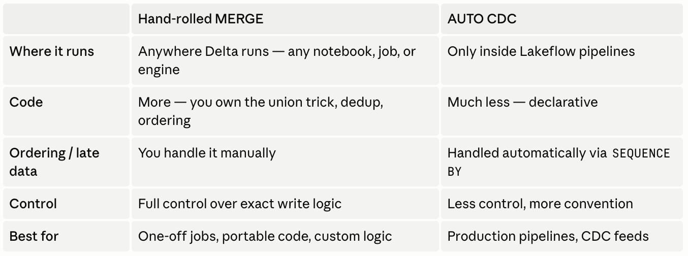
My rule of thumb: if you are already building a Lakeflow pipeline, use AUTO CDC — it removes a whole category of bugs around ordering and duplicate keys. If you need something portable, ad-hoc, or with custom write logic, use MERGE. Knowing both makes you dangerous in the best way, because you can pick the right tool instead of forcing one pattern everywhere.

Type 1 vs Type 2, Side by Side

Let me make the difference visceral with one event. A customer, ID 100, is currently in Kyiv. An update arrives: they moved to Lviv.

With SCD Type 1, after the MERGE, the table has one row:

Kyiv is gone. If someone asks where customer 100 lived last year, you cannot answer. You traded history for simplicity.

With SCD Type 2, after the operation, the table has two rows:

Now the full story is preserved. You can join a fact table to the version that was current at any point in time. This is why Type 2 is the backbone of proper data warehousing — and why choosing Type 1 by accident, when you needed history, is such a costly mistake.

Same source event. Completely different capability. That is the decision SCD is really about.

Common Mistakes to Avoid

• Using Type 1 when you needed history. This is the big one, and it is irreversible. Once you overwrite, the old values are gone forever. When in doubt about whether history matters, use Type 2 — you can always ignore history, but you cannot recover what you never kept

• Not deduplicating the source before MERGE. Multiple changes for one key in a single batch will error or apply out of order. Deduplicate to the latest record per key first

• Forgetting to close the old row in Type 2. If you insert the new version without setting the old row’s current flag to false and its end date, you end up with two “current” rows per key and broken queries

• Confusing the business key with the surrogate key. In a Type 2 table, the business key (customer_id) repeats across versions. Use a separate surrogate key as the unique row identifier

• Hand-rolling MERGE ordering when AUTO CDC would do it for you. If you are in a Lakeflow pipeline fighting with out-of-order events, `SEQUENCE BY` solves it in one line
  Reaching for APPLY CHANGES in new code. It still works, but AUTO CDC is the current, recommended API. Learn the new one

Frequently Asked Questions

What is a slowly changing dimension?

A slowly changing dimension is a dimension table whose attributes change over time, together with the strategy you use to handle those changes. The main question it answers is whether you overwrite old values (no history) or preserve them (full history).

What is the difference between SCD Type 1 and Type 2?

SCD Type 1 overwrites the old value with the new one, keeping no history — your table always shows only the current state. SCD Type 2 keeps every version as a separate row with a start date, end date, and current flag, so you preserve the full history and can answer point-in-time questions. Type 1 is simpler; Type 2 is auditable.

How do I implement SCD Type 2 in Databricks?

Two ways. With MERGE, you use a “union trick” — stage two copies of each changed record, one that closes the old row and one that inserts the new current row. With AUTO CDC in a Lakeflow pipeline, you declare `STORED AS SCD TYPE 2` and it handles the history columns, ordering, and deletes for you.

What replaced APPLY CHANGES on Databricks?

AUTO CDC. The AUTO CDC APIs replace APPLY CHANGES and use the same syntax. APPLY CHANGES still works, but Databricks recommends AUTO CDC (`AUTO CDC INTO` in SQL, `create_auto_cdc_flow` in Python) for new code.

Should I use MERGE or AUTO CDC for SCD?

Use AUTO CDC when you are building a Lakeflow pipeline — it is declarative and handles ordering and late data automatically. Use MERGE when you need portable code that runs anywhere Delta runs, or when you want full control over the exact write logic.

Why does SCD Type 2 need two rows for one change?

Because a change means one version ends and another begins. The old row is closed (current set to false, end date filled in) so it becomes history, and a new row is inserted (current true) to represent the new state. Two rows, one per version, is what preserves the timeline.

What Is Next

You now know how to keep history in your dimension tables — the pattern that separates a toy warehouse from a real one. In the next article, we tackle a related essential: schema enforcement and evolution in Delta Lake— how Delta protects your tables from bad data, and how to change your schema safely when your data genuinely evolves.

Make sure to bookmark this series so you do not miss any upcoming articles.

Want more? Visit mbvyn.com for mentorship, consulting, and all my content in one place. And if you work with Parquet files, try parquetreader.app — my free tool for exploring them in your local environment.